
Scaling reinforcement learning with verifiable rewards for LLMs on LUMI
15 mins read
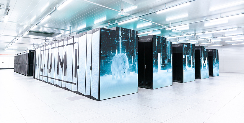
A supercomputer such as LUMI consists of many compute nodes that can work together to solve large computational problems. Adding nodes can help complete a task faster or make it possible to process a larger workload, but the benefit depends on how efficiently the added resources are used. This is known as scaling.
Using a large language model (LLM) training workload as an example, this technical blog post explains different types of scaling, what can affect performance, and how to measure whether additional resources are useful. While your own AI workload might differ, many of the same principles still apply.
Reinforcement learning (RL) has become a vital method for post-training LLMs, particularly to improve their reasoning and problem-solving abilities. While scaling of LLM pre-training has previously been studied on the LUMI supercomputer, there appears to be little published work on scaling RL. We use the open-source framework verl to study how RL post-training scales from one to 16 nodes on LUMI-G, LUMI’s GPU partition. Our findings provide academic and industry users with a practical foundation for further reinforcement learning experimentation on LUMI.
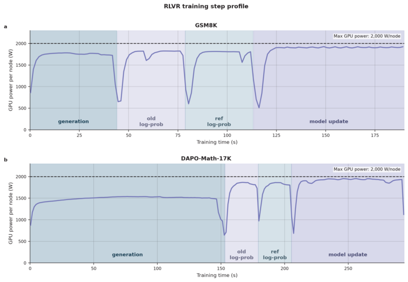
In the reinforcement learning with verifiable rewards (RLVR) paradigm, the outputs of the model are checked automatically, and the model is updated based on the feedback. For example, a mathematical answer can be checked against an exact solution, or a coding task succeeds if all unit tests pass. RLVR presents a very different systems workload from pre-training: instead of repeatedly training on existing batches of text, a synchronous¹ RLVR step alternates between inference and training. During generation, the model produces one or more responses for each prompt. Each prompt-response pair forms a trajectory, which receives a reward based on its outcome. These rewards are then used to construct the loss for updating the model. Figure 1 shows these phases from a complete RLVR training step for two different datasets. A pre-training step would most closely resemble the model update phase.
¹ Synchronous: the model update waits until every generation in the current batch is finished, so training data always matches the current version of the model, but some GPUs may idle waiting for the slowest response. Asynchronous: generation and model updates overlap, which reduces GPU idling, but some answers may have been generated by a slightly older version of the model.
We chose verl because it supports various existing LLM frameworks for training (e.g., Megatron, FSDP) and inference (e.g., vLLM, SGLang), while having a broad coverage of RL algorithms. We use the Qwen3-8B model and the group relative policy optimization (GRPO) algorithm (see “The GRPO algorithm in a nutshell” below) in the scaling experiments.
Each LUMI-G GPU node contains four AMD Instinct MI250X accelerators and one 64-core CPU. The MI250X GPU is a multi-chip module with two GPU dies, called Graphics Compute Dies (GCDs), each with access to 64 GiB of memory. Because every GCD is exposed as an independent device, software detects eight GPUs per node. For the purposes of this post, we will refer to GCDs as GPUs. The complete software environment and training scripts used to reproduce this study are available in the GitHub repository. Examples for getting started with RLVR training on LUMI using the available LUMI AI Factory (LUMI AIF) containers are available in the CSC GitHub repository.
The GRPO algorithm in a nutshell:
This brief introduction provides background needed to understand our scaling experiments. For a detailed description of the algorithm, see the original DeepSeekMath paper.
1. The model generates a group of answers for each prompt in the training batch. In our experiments, each group contains eight answers. The total number of generated trajectories is prompts × answers per prompt. This is the generation phase in Figure 1.
2. A reward function scores the model’s answers. GRPO compares the scores within each group, encouraging answers that score better than the group average and discouraging those that score worse.
3. GRPO recomputes the token probabilities for the generated answers using the model that generated them, and a fixed reference model from before RL training began. These calculations help keep the model update controlled. These are the old log-prob and ref log-prob phases in Figure 1.
4. The reward scores and recomputed token probabilities are used to compute the loss. The loss is then used to update the model weights. This is the model update phase in Figure 1.
How we measured the scaling of our workload
The profile of a reinforcement learning step depends on many variables, including the model, dataset, and response-length limit. Different prompts produce responses of different lengths, which affects both the optimal training configuration and the balance between generation and model updates (see Figure 1).
For our scaling experiments, we chose the Qwen3-8B model as a representative open-weight reasoning model in the 8B parameter class. All experiments use GRPO with eight answers per prompt, vLLM for generation, Megatron for training, and the AdamW optimiser. Training uses tensor parallelism (TP) of 8, giving data parallelism (DP) of 1 on one node; TP4 was slightly faster on one node but failed during multi-node initialisation on our software stack. Generation uses node-local TP4/DP2, which is the fastest rollout configuration tested.
To study two different workload regimes, we use the GSM8K and DAPO-Math-17K math datasets. GSM8K contains, on average, easier questions and produces shorter responses, whereas DAPO-Math-17K problems are more difficult, and the model tends to generate much longer responses. We set the response caps to 1,024 tokens for GSM8K and 8,192 tokens for DAPO-Math-17K. Approximately half of the generated responses reach the response cap in both workloads. With these configurations, generation takes about one quarter of a GSM8K training step and half of a DAPO-Math-17K step.
Our main metric is throughput: the total number of prompt and response tokens in the generated trajectories, divided by the complete step time and number of GPUs. Each token is counted once, even though the trajectory is processed again during the log-probability and model update phases. Unlike pre-training throughput, which measures model training alone, our metric covers the complete RLVR step, including generation and log-probability recomputation.
Each reinforcement learning training run contains 20 steps. We report the mean and sample standard deviation of steps 2–20, excluding the first step as warm-up. We set the learning rate to zero to prevent model updates from changing the response distribution during measurement. The complete forward, backward, and optimiser steps are still executed, but the model weights do not change. Due to sampling, realised token counts can vary slightly between steps. However, the mean realised workload remained close to the intended at each scale, so differences in generated token counts do not explain the observed scaling results.
Weak scaling: Increasing the workload and the computational resources simultaneously
Weak scaling asks whether the system can process a proportionally larger workload as more resources are added. For weak scaling, we first found an approximately throughput-optimal one-node workload for both datasets and then increased both the node count and prompt batch size proportionally from one to 16 nodes. The other training settings were kept fixed.
Selecting the one-node workloads for both datasets was primarily a question of how much GPU memory to allocate to generation concurrency (how many answers GPUs generate simultaneously). We matched the generation concurrency to the number of trajectories, allowing all answers of a training step to be generated at the same time. If the concurrency was lower than the number of trajectories, some answers would begin only after earlier answers had finished, doubling generation time in the worst case. Concurrency higher than trajectory count would not improve performance because all answers could already be generated simultaneously.
We increased the prompt count and generation concurrency together until throughput stopped improving or GPU memory was exhausted. We selected the one-node configurations such that peak GPU memory use during training stayed below approximately 98% of the available 64 GiB per GPU.
For GSM8K, the benefit from additional concurrency saturated at 100 prompts, or 800 trajectories, before GPU memory became the limiting factor. Increasing the prompt count further raised the memory demand without improving throughput. The available memory was instead used to accelerate training: activation recomputation and CPU offloading were disabled, and a larger gradient accumulation batch token budget was chosen.
For DAPO-Math-17K, long responses kept generation dominant, and throughput continued to benefit from greater concurrency. We therefore enabled activation recomputation and CPU offloading and used a smaller gradient accumulation batch token budget to free more GPU memory for generation. This resulted in a one-node workload of 10 prompts, or 80 trajectories. The selected one-node configurations and measured workload characteristics are summarised in Table 1.
Table 1: Selected one-node configurations for GSM8K and DAPO-Math-17K. In weak scaling, the number of prompts is increased proportionally to nodes. The fixed strong scaling workloads contain four times the prompts and trajectories shown here.
| One-node workload profile | GSM8K | DAPO-Math-17K |
| Model | Qwen3-8B | Qwen3-8B |
| Algorithm | GRPO | GRPO |
| Training / rollout backend | Megatron / vLLM | Megatron / vLLM |
| Training / rollout precision | BF16 / BF16 | BF16 / BF16 |
| Optimiser | AdamW | AdamW |
| Learning rate | 0 | 0 |
| Token caps (prompt / response) | 256 / 1,024 | 381 / 8,192 |
| Prompts / answers per prompt / trajectories | 100 / 8 / 800 | 10 / 8 / 80 |
| Mean response length¹ | 869 tokens | 6,879 tokens |
| Responses reaching the cap¹ | 51.2% | 52.2% |
| Total tokens / step¹ | 761k | 562k |
| Actor / reference parallelism | TP8 / DP1 | TP8 / DP1 |
| Actor DP sharding | ZeRO-1 | ZeRO-1 |
| Rollout parallelism | TP4 / DP2 | TP4 / DP2 |
| Rollout engines | 2 | 2 |
| Concurrency / rollout engine | 400 | 40 |
| Generation share of training time¹ | 22.9% | 51.6% |
| Microbatch token budget / GPU² | 12,288 | 9,472 |
| Training memory strategy | no recomputation or CPU offload | full recomputation and parameter, gradient and optimiser offload |
¹ Mean over steps 2–20 of the one-node run. ² Dynamic-batching token budget used for model updates and old-policy/reference log-probability passes.
These per-node workloads were scaled across 1, 2, 4, 8, and 16 nodes. In weak scaling, the GSM8K workload therefore grew from 800 to 12,800 trajectories per step, and the DAPO-Math-17K workload grew from 80 to 1,280 trajectories.
Strong scaling: Keeping the workload fixed and adding more computational resources to complete it faster
Strong scaling analyses are used to determine how much a fixed workload can be accelerated by adding more resources. Choosing the workload solely on maximum throughput would favour large batches, which provide more parallel work and amortise fixed costs. However, batch size is also an algorithmic choice that can affect sample efficiency and convergence, so it cannot be selected on throughput alone. We therefore reviewed workloads used in RL literature and selected realistic workloads from our weak scaling series to be used in strong scaling.
The reviewed studies use approximately 256–8,192 trajectories per step. For DAPO-Math-17K, 512 trajectories is a recurring choice. For GSM8K, reported workloads vary more widely, with no clearly recurring configuration, so we selected a workload near the middle of the range. Based on this, we chose the four-node weak scaling workloads for the strong scaling study: 400 prompts × 8 answers = 3,200 trajectories for GSM8K and 40 prompts × 8 answers = 320 trajectories for DAPO-Math-17K. Choosing the four-node workloads allows us to have two measurements above and below the four-node point.
These workloads were held fixed, and we ran them on 1, 2, 4, 8, and 16 nodes. The four-node run is shared with the weak scaling series. At higher node counts, each rollout engine handles fewer trajectories and requires less generation memory. This memory could potentially speed up training by using fewer gradient accumulation steps or less activation recomputation and offloading. Tuning the settings for each node count might improve individual results, but a separate configuration search was not practical for this study.
How RLVR scales from one to 16 LUMI-G nodes
Figure 2 shows that weak scaling efficiency at 16 nodes is 77.9% for GSM8K and 96.1% for DAPO-Math-17K. Although DAPO-Math-17K has lower absolute throughput, it retains per-GPU performance much better as the system grows. GSM8K efficiency declined approximately linearly by about 1.4 percentage points per added node, while DAPO-Math-17K remained within four percentage points of its one-node efficiency.
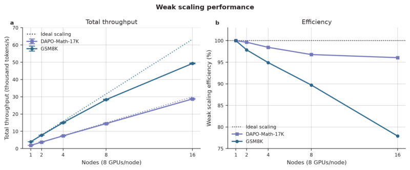
Workload granularity likely explains part of the difference. At every node count, GSM8K processes ten times more trajectories than DAPO-Math-17K, 12,800 trajectories versus 1,280 at 16 nodes. This may increase scheduling, scoring, and data-processing overhead. DAPO-Math-17K’s longer trajectories also keep each GPU busy for longer and better amortise these costs. However, the workloads differ in several other respects, including their prompt and response distributions, training step profiles, trajectory scoring, scheduler concurrency, and GPU memory configurations. The results therefore compare two different workload regimes, not the isolated effect of trajectory length.
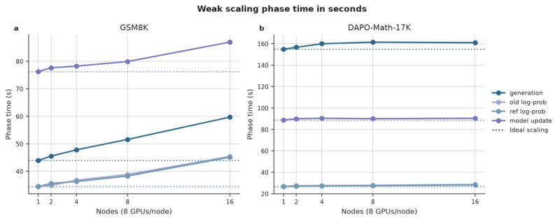
Figure 3 shows how the main phase times of a training step change during weak scaling. In ideal scaling, the phase times would stay constant when proportionally increasing the workload and the resources, as per node work stays the same. For DAPO-Math-17K, the phase times remain nearly constant, and the complete step grows by only 12.3 seconds (4.1%) from 1 to 16 nodes. The GSM8K step grows by 55.6 seconds (28.9%) over the same range, and the additional time is distributed across the main phases rather than concentrated in any single phase.
For strong scaling, we use the four-node workloads from the weak scaling study, as described previously. Therefore, all speedups are measured relative to the four-node time. Figure 4 shows two scaling regimes: performance changes nearly proportionally to the resources between one and four nodes and adding nodes beyond four gives diminishing returns. From four to 16 nodes, GSM8K step time decreases from 204 to 72 seconds, a 2.8× speedup. DAPO-Math-17K decreases from 309 to 165 seconds, a 1.9× speedup. The ideal speedup is 4×.
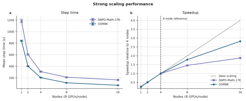
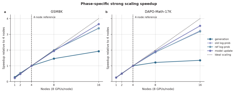
Figure 5 helps explain the diminishing returns. At four nodes, each rollout engine receives a full batch of trajectories. At one and two nodes, generation scales efficiently as continuous batching keeps the engines saturated while they process the trajectories in multiple waves. Above four nodes, the fixed workload is divided among more engines, leaving them underfilled. At 16 nodes, each engine processes 100 GSM8K trajectories or only 10 DAPO-Math-17K trajectories, compared with 400 and 40 at four nodes. Generation continues to become faster, but scales less efficiently than the model update and log-probability recomputation phases. Compared with ideal scaling from four to 16 nodes, generation accounts for about 60% of the extra GSM8K step time and 90% of the extra DAPO-Math-17K step time.
As the per-engine workload decreases, some GPU memory reserved for generation could instead be used to accelerate log-probability computation and model updates. At 16 nodes, these phases take about 43 seconds for both datasets and account for 60% of the GSM8K step but only 26% of the DAPO-Math-17K step. A speedup of these phases would thus have a larger effect on the complete GSM8K step, while DAPO-Math-17K would still be dominated by generation.
Conclusions
We demonstrated synchronous Qwen3-8B RLVR training with verl on up to 16 LUMI-G nodes. At 16 nodes, DAPO-Math-17K retained 96.1% weak scaling efficiency and GSM8K 77.9%. Strong scaling was close to ideal up to four nodes, but beyond that generation engines received too little work to benefit fully from additional nodes.
Key takeaways:
- RLVR alternates between inference and model training, making it a different workload from the more uniform pre-training loop.
- RLVR workloads can behave very differently. In our study, generation occupied about one quarter of the GSM8K step with its many short trajectories, but half of the DAPO-Math-17K step with its fewer, much longer trajectories.
- Effective RLVR optimisation requires an understanding of the complete training step and the interactions between its phases. GPU memory saving techniques in training improved the generation dominated DAPO-Math-17K workload but were not beneficial for GSM8K.
- LUMI AIF containers provide an optimised software environment for LUMI’s GPUs and the high-speed network. In many cases only a few project-specific packages need to be added, such as verl in our case.
This study covers synchronous RLVR training with two different workloads and a frozen-weight model. Other models, datasets, and training pipelines, including asynchronous approaches, may behave differently. Nevertheless, the validated software environment, workload configurations, and scaling measurements establish a foundation for further RLVR experimentation on LUMI. To try RLVR yourself, check out our RLVR examples for LUMI, or the resources to reproduce this scaling study.
Read also other blogs in the series:
What is LUMI AI Factory’s Artificial Intelligence expert consultation?
Written by

Markus Junttila
Trainee in AI and Data Analytics

Gaurav Naithani
Machine Learning Specialist

Marlon Tobaben
Machine Learning Specialist